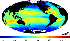
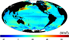
Notable features of the 1° OAFlux analysis:

The 1° OAFlux analysis is constructed from using the best possible surface meteorological variables and best possible bulk flux algorithm. Buoy measurement time series at 130+ buoys are used as independent benchmark for validating the estimated air-sea variables; these buoys are not assimilated in the OAFlux synthesis process (Yu and Weller 2007; Yu et al. 2008).

• The best possible estimates for flux-related surface meteorological variables are obtained by applying an advanced objective analysis to seek optimal synthesis of satellite observations of wind speed and SST and atmospheric reanalysis of near-surface air and humidity. The latter two variables cannot be directly observed by satellite so auxiliary datasets have to be supplied to complete the flux estimates. In OAFlux 0.25° satellite analysis, the two variables are retrieved from satellite microwave radiometers and sounders (Yu and Jin 2018), which is one main difference between the two versions of products.

• The objective analysis denotes the process of synthesizing measurements/estimates from various sources. The methodology governing the objective analysis is the Gauss – Markov theorem, a standard statistical estimation theory that states, when combining data in a linear fashion, the linear least squares estimator is the most efficient estimator. Such process reduces error in each input data source and produces an estimate that has the minimum variance. That means that the OAFlux analysis takes data errors into account when constructing improved estimates of flux-related surface meteorological variables.

• The latent and sensible heat flux estimates are computed from the objectively analyzed surface meteorological variables by using the COARE bulk flux algorithm 3.0 (Fairall et al. 2003).