Two versions (1° & 0.25°) of OAFlux products: What are the differences?
Surface turbulent momentum fluxes, latent and sensible heat fluxes, and moisture flux (or ocean evaporation) over the global ocean cannot be directly observed from either satellite or in situ sensors. These fluxes are estimated using the following bulk flux parameterizations:
τx = ρ Cd |W - Ws| (u - us) (1)
τy = ρ Cd |W - Ws| (v - vs) (2)
QLH = ρ Lv CE |W - Ws| (qs - qa) (3)
QSH = ρ cp CH |W - Ws| (Ts - Ta) (4)
E = QLH/(ρwLv) (5)
where τx and τy are the respective zonal and meridional wind stress components, QLH the latent heat flux, QSH the sensible heat flux, and E the moisture flux. The input variables for calculating the fluxes (1)-(5) are the zonal (u), meridional wind (v) components, and wind speed (W) at a reference height, the ocean-surface current velocity (us, vs) and speed (Ws), sea-surface temperature (SST, Ts), the potential air temperature (Ta) and specific humidity (qa) at a reference height, and saturation specific humidity (qs) as a function of Ts and sea level pressure. The other constants are ρ the air density, ρw the sea-water density, Lv the latent heat of vaporization that is expressed as Lv = (2.501 – 0.00237×Ts)×1.06, and cp the isobaric specific heat. The turbulent transfer coefficients, Cd, CE, and CH, depend on wind speed, atmospheric stability, measurement height, surface roughness, surface wave height and wave age.
At OAFlux, efforts are made to improve the accuracy of surface fluxes through improving the accuracy of flux-related input variables. We utilize the state-of-art approaches including machine learning tools to derive insights from satellite and in situ observations in developing the best strategy for extracting and merging air-sea variables from satellite active and passive sensors (including scatterometers, radiometers, and sounders).
Two versions of OAFlux products have been developed. The first one is the 1°-gridded analysis of 60+ years that has been available online since 2008 under the auspices of the NOAA Global Ocean Monitoring and Observing Program. This version of analysis is constructed from objective synthesis of satellite observations of wind and sea surface temperature and atmospheric reanalysis output of near-surface air temperature and humidity. Air-sea measurement time series from moored buoys at 130+ locations are used as benchmark for calibration and validation. The second version is the new, high-resolution (HR; 0.25°-gridded) analysis of the satellite era (1988 - present, 30+ years) sponsored by NASA Making Earth System Data Records for Use in Research Environments (MEaSUREs) Program. This OAFlux-HR analysis is all satellite-based, with near-surface air humidity and temperature retrieved from 11 microwave radiometers and sounders and vector winds merged from 16 scatterometers and radiometers. In summary, the two versions of OAFlux products are developed from two different and independent methodologies. Major features of the two versions of products are listed in Table 1, and the differences in the resulting fluxes are shown Figures 1-2.
Table 1. Methods used in Developing OAFlux 1° and OAFlux 0.25°.

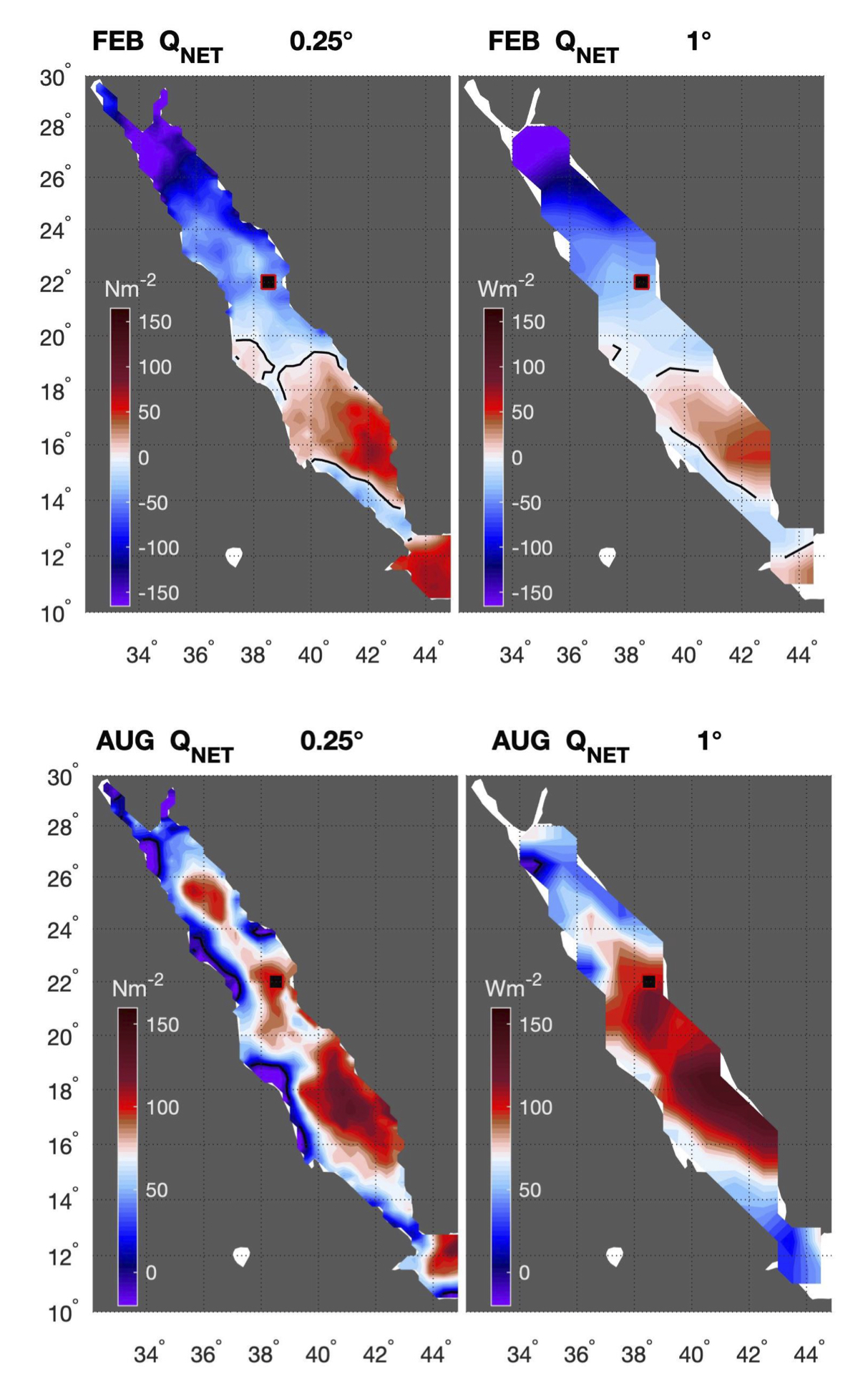
Figure 1. Snapshots of net heat input into the Red Sea (Qnet, unit: W/m². positive downward) produced by OAFlux-0.25° analysis (left) and OAFlux-1° analysis (right) in February (top) and August (bottom). Qnet is the sum of solar radiation, longwave radiation, turbulent latent and sensible heat fluxes. The OAFlux higher-resolution flux analysis provides a more detailed depiction of the orographical influence on spatial variability of air-sea fluxes. The Red Sea is a semi-enclosed marginal sea of the North Indian Ocean, lying between Asia and Africa. The region has experienced significant warming in recent decades and an abrupt shift in surface winds in the late 1990s. An accurate quantification of Qnet is essential for understanding the responses of the Red Sea's weather and climate to the global-scale climate warming.
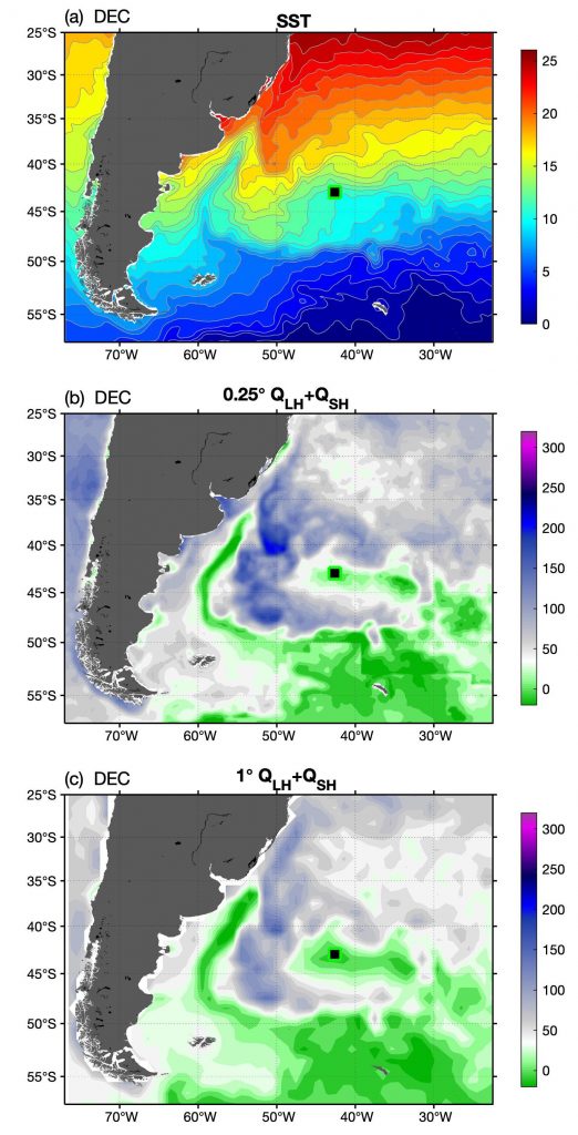
Figure 2. December snapshot of (a) sea surface temperature SST, and turbulent heat loss (QLH+QSH; unit: W/m²; positive upward) produced by (b) OAFlux-0.25° analysis and (c) OAFlux-1° analysis in the Brazil - Malvinas confluence zone. SSTs shaded in bluish colors are associated with the cold Malvinas Current (also called Falkland Current) and those in reddish colors associated with the warmer Brazil Current. Note that the OAFlux-0.25° analysis has a better representation of the tight air-sea flux frontal structure induced by the equatorward intrusion of the Malvinas Current along the shelf break.